

Exponentially Weighted Moving Average Research
Содержание статьи:
Volatility is the most common way to measure risk, but it also comes in several shades.
In the previous article, we figured out how to calculate simple historical volatility .
Read also
Volatility. Financial market volatility indicators
What is the relationship between market liquidity and volatility?
In this article, we will make simple volatility corrections and discuss Exponentially Weighted Moving Average (EWMA).
Historical and implied volatility
First, let’s take a detached look at these parameters. There are two popular approaches: historical and implied (or implicit) volatility.
The historical approach assumes that the past is a prologue to the present; analysts measure historical data in the hope that it has predictive value.
On the other hand, implied volatility ignores history; in this case, the volatility forecast is driven by current market prices.
At the same time, analysts hope that the market knows everything better, and that the market price contains a consensus estimate of volatility, albeit indirectly.
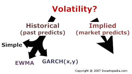
If we focus only on three historical approaches (in the illustration on the left), then you can see two common stages in them.
- Calculation of a series of periodically repeating deviations.
- Application of the scheme for adding weighting factors.
First, we calculate the periodic deviations. This is usually a series of deviations over the course of the day, where results are constantly being combined.
For each day, a record of the share price ratio is used (that is, today’s price is divided by yesterday’s, and so on).
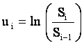
This gives a series of daily deviations from u i to u i-m , depending on how many days (m = days) we are measuring.
This brings us to the second stage. Here these three approaches differ from each other.
In the previous article, we showed that, given a few acceptable simplifications, the simple variance is the mean squared deviation:
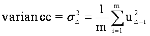
Note that this adds up each of the periodic deviations, and then divides that total by the number of days or observations (m).
Thus, this is just the mean of the squares of the periodic deviations. In other words, equal weight is assigned to all squares of deviations.
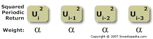
Therefore, if the coefficient alpha (a) is a weighting factor (for example, a = 1 / m), then the simple variance looks like this:
EWMA corrects the shortcomings of simple variance.
The weakness of this approach is that all deviations are given the same weight.
Yesterday’s (very recent) value has no more impact on variance than last month’s results.
This problem is solved by using an Exponentially Weighted Moving Average (EWMA), in which later values are weighted more for the variance.
The Exponentially Weighted Moving Average (EWMA) introduces a lambda parameter , also called a smoothing parameter. The lambda value must be less than one.
In this case, instead of equal weighting factors, each square of the deviation is weighted using a special multiplier as follows:
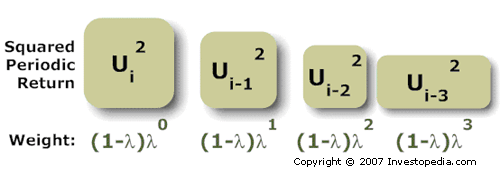
For example, a company of RiskMetrics TM , which is engaged in financial risk management, usually uses ” lambda ” 0.94, or 94%.
In this case, the coefficient (1-0.94) (0.94) 0 = 6% is assigned to the first (most recent) square of the periodic deviation .
The next square of the deviation is simply the lambda factor of the previous weight; in this case 6% is multiplied by 94% = 5.64%. And the weight of the third day is (1-0.94) (0.94) 2 = 5.30%.
This is the meaning of the term ” exponential ” in EWMA: the weight of each day is a fixed factor (ie lambda, which must always be less than one) of the weight of the previous day.
This allows the variance of the score to be weighted or biased towards more recent data. (To learn more, check out the Google Volatility Excel Sheet.)
The difference between simple volatility and EWMA in the case of Google is shown below.
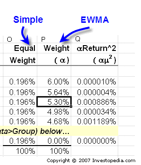
When calculating simple volatility, each periodic deviation is weighted 0.196%, as shown in column O (we had two years of stock price data for each day.
That is, 509 daily deviations, so 1/509 = 0.196%). But notice that in column P, the items are weighted 6%, then 5.64%, then 5.3%, and so on.
This is the only difference between simple variance and EWMA.
Remember: after adding up the entire series (in column Q), we get the variance, which is the square of the standard deviation.
If we need to calculate volatility, we will need to take the square root of this variance.
What is the difference in daily volatility between variance and EWMA in Google’s case?
This is important to consider: a simple variance shows us a daily volatility of 2.4%, but the EWMA shows a daily volatility of only 1.4% (see the table for details).
Google’s volatility seems to have calmed down quite recently, so the high simple variance is artificial.
Today’s variance is derived from the variance of the previous day
You might have noticed that we need to compute a long series of exponentially decreasing weights.
We won’t do the math here, but one of the best things about EWMA is that the entire series can be conveniently reduced to a recursive formula:
![]()
The term ” recursive ” means that today’s variance depends on the variance of the previous day (that is, it is a function of it).
You can also find this formula in spreadsheets and it gives the same result as long manual calculations!
It says: today’s variance (by EWMA) is equal to yesterday’s variance (weighted ” lambda “) plus yesterday’s squared deviation (weighted ” one minus lambda “).
Note that we have simply combined two terms: yesterday’s weighted variance and the square of yesterday’s weighted variance.
However, ” lambda ” is an anti-aliasing parameter.
A higher lambda (eg 94% like RiskMetric) indicates a slower decay in the series – in relative terms, we will have more data points in the series, and they will decrease more slowly.
On the other hand, if we decrease the lambda , we get a higher roll-off rate: the weights decrease faster and, as a direct result of the fast roll-off, fewer data points are used.
(In a spreadsheet, ” lambda ” is an input parameter, so you can experiment with its sensitivity).
Outcome
Volatility is the instantaneous standard deviation of a stock and is the most common way to measure risk.
It also represents the square root of the variance. Variance can be measured historically or implicitly (implied volatility).
When measured historically, simple variance is the most popular method.
But the weakness of using simple variance is that all variances are weighted equally.
Thus, we are faced with a classic trade-off: we always want to have more data, but the more we use the data, the more our calculations are diluted with remote (less relevant) data.
Exponentially Weighted Moving Average (EWMA) corrects simple variance problems by weighting individual periodic deviations.
This way we can use a larger sample size, but also give more weight to relatively recent results.